Ch.66: K-Means Clustering, the Geometric Intuition

By Ayush Arora•2026-10-02•10 min read

Inspired by: YouTube

1. Clustering: Grouping Without Labels

Every algorithm covered so far in this series has been supervised: the training data comes with an answer column, and the model's job is to learn the mapping from inputs to that answer. Clustering is different. There's no answer column at all, just points, and the job is to group similar points together. An e-commerce company clusters customers to target them differently; a college clusters students to prepare them differently; an image pipeline clusters pixels or image embeddings to segment a photo. None of these come with a ground-truth "correct group" label to train against, which is exactly what makes this unsupervised learning.

K-means is the most common clustering algorithm, and a specific problem makes a good entry point into it: a college's placement cell has CGPA and IQ for its final-year CSE students and wants to group them so each group can be prepped differently for interviews.

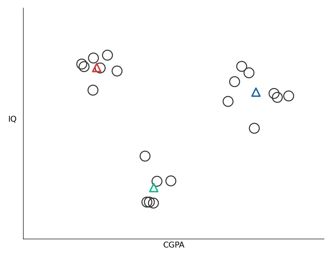
Scatter plot of CGPA against IQ with 21 outlined circular points. The points visually separate into three distinct groups: one upper-left, one lower-middle, one upper-right. A colored triangle (red, teal, blue respectively) sits near the center of each group.

Plotted on two axes, this is almost insultingly easy: a human eye immediately sees three groups, and it's obvious which point belongs to which. That ease is the trap. Real student data has far more than two columns, 10th-grade marks, 12th-grade marks, city, family income, a dozen other fields, and once there are more than two or three dimensions, nobody can eyeball "three groups" on a plot that doesn't exist. The entire point of K-means is to do algorithmically, in any number of dimensions, what the eye just did for free in two.

2. The Algorithm Works the Same in 2D and in 100D

This post sticks to two dimensions throughout, CGPA and IQ, purely so every step can be drawn. But nothing about the algorithm below is specific to 2D; the same five steps run unchanged whether there are 2 input columns or 200. That's the actual value of K-means: most real clustering problems involve more columns than anyone can visualize, and this is one of the few algorithms that doesn't care.

3. The One Weird Requirement: You Choose K Yourself

Before describing the steps, one uncomfortable fact needs to be stated up front. K-means cannot figure out on its own how many clusters a dataset has. The $K$ in "K-means" is a number the programmer supplies, not something the algorithm infers from the data. Looking at a 2D plot, a person can decide "this looks like 3 groups," but K-means has no equivalent instinct, and in high-dimensional data where nobody can plot anything, this becomes a genuinely tricky question. It has a real answer (Section 6), but it's worth sitting with the discomfort first: an algorithm whose first input is a number nobody can derive from first principles, only estimate.

For this dataset, assume the answer is decided to be $K=3$ .

4. The Algorithm, Step by Step

With $K$ fixed, K-means runs five steps, the first two happening once and the last three repeating in a loop:

Decide $K$ (done above: $K=3$ ).
Initialize $K$ centroids at random positions. A centroid is just a point in the same space as the data, meant to eventually sit at the center of a cluster, but at this stage it's placed with no information about where the real clusters are.
Assign every point to its nearest centroid, measuring distance with the ordinary Euclidean distance formula. Each point now belongs to whichever of the $K$ centroids it's closest to.
Move each centroid to the mean of the points now assigned to it. A cluster's centroid is recomputed as the average CGPA and average IQ of its current members, which usually shifts the centroid's position.
Check whether anything changed. If a centroid moved in step 4, the cluster memberships from step 3 may no longer be optimal (some points might now be nearer a different centroid), so go back to step 3 and reassign. If no centroid moved, the assignments are stable and the algorithm stops.

The buttons below step through an actual run of this loop, on the same 21-student dataset shown in Section 1. Click through them in order; each one carries the same point data and simply re-assigns colors and moves the triangles:

4.1 Random Initialization

A common way to initialize centroids, and the one used here, is to pick $K$ actual data points at random and use their coordinates as the starting centroids, rather than inventing arbitrary coordinates from nowhere. Three students get selected this way, and their (CGPA, IQ) values become the three starting centroids, not necessarily anywhere near where the real cluster centers will turn out to be. Every point is still gray, since nothing has been assigned to anything yet.

4.2 Round 1: Assign, Then Move

Every point computes its Euclidean distance to all three centroids and joins whichever is closest. Once every point has a color, each centroid relocates to the mean position of its own color. The green and blue centroids move only slightly, since the random initialization happened to land close to their eventual clusters; nothing here depends on that being true in general, it's simply what this particular random start produced.

4.3 Round 2: A Correction

Because the centroids moved, step 5 sends the algorithm back to step 3: distances are recalculated against the new centroid positions, and this time one student switches which cluster they belong to, since their nearest centroid changed once the centroids shifted. This is the mechanism doing real work: a point's cluster assignment isn't fixed at step 3, it keeps getting re-evaluated every round, and it's entirely possible for a point to flip clusters partway through, even though the data itself never changed, because the frame of reference (the centroids) did.

4.4 Convergence

With that student reassigned, the centroids move again to the new per-cluster means, and the loop returns to step 3 one more time. This round produces no reassignments at all, every point is already closest to the correct centroid, so step 4 leaves every centroid exactly where it was. Since nothing changed, step 5's check says the algorithm is done, landing on the same three clusters a human eye picked out instantly in Section 1, starting from centroids that began nowhere near them.

4.5 Why Euclidean Distance Specifically

The entire algorithm rests on one geometric operation, measuring the distance between two points, and Euclidean distance is what's used:

d(p, q) = \sqrt{\sum_{i=1}^{n} (p_i - q_i)^2}

The useful property here isn't anything exotic, it's that this formula is defined identically for 2 dimensions, 3 dimensions, or 300. The same assign to nearest centroid step that worked on the CGPA/IQ plot above runs unchanged on a 300-column dataset; only the number of terms under the square root changes. That portability is a direct answer to Section 2's claim: K-means scales to high dimensions because its one geometric primitive scales to high dimensions.

5. Picking K: The Elbow Method

Section 3 left a real question unanswered: where does $K=3$ actually come from, beyond "it happens to look right in 2D"? The standard answer is the elbow method, built around a quantity called WCSS (within-cluster sum of squared distances), also called inertia.

For a single cluster with centroid $c$ and member points $p_1, \ldots, p_m$ , that cluster's WCSS is:

\text{WCSS}_{\text{cluster}} = \sum_{j=1}^{m} d(p_j, c)^2

the sum of each point's squared distance to its own centroid. A dataset's overall WCSS for a given $K$ is just the sum of this quantity across all $K$ clusters. The elbow method's recipe: run K-means for $K = 1, 2, 3, \ldots$ up to some reasonable cap, record the overall WCSS at each $K$ , and plot $K$ against WCSS.

Two boundary cases pin down the shape of that curve before looking at any actual numbers. At $K=1$ , every point belongs to one giant cluster, so WCSS is as large as it can get. At $K = n$ (as many clusters as points), every point is its own centroid, every distance is exactly 0, and WCSS is exactly 0. Between those two extremes, WCSS strictly decreases as $K$ grows, more clusters can only ever reduce or match the total squared distance, never increase it.

Running this on the placement dataset for $K=1$ through $K=8$ :

Line chart with number of clusters K on the x-axis (1 through 8) and WCSS on the y-axis. The curve drops steeply from K=1 to K=3, then flattens out almost completely from K=3 onward. A red circle and annotation mark K=3 as the elbow point.

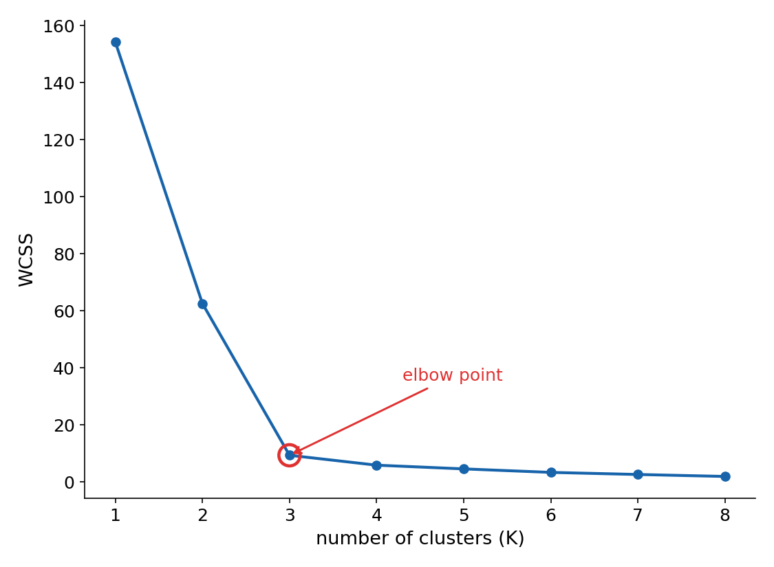
The WCSS values themselves make the shape concrete: 154.3 at $K=1$ , 62.6 at $K=2$ , 9.4 at $K=3$ , then 5.9, 4.6, 3.4, 2.7, 1.99 for $K=4$ through $K=8$ . The drop from $K=1$ to $K=3$ is enormous; the drop from $K=3$ onward is comparatively tiny. That's the elbow point: the $K$ where adding another cluster stops buying much reduction in WCSS. Visually, it's where the curve's steep decline flattens into a near-plateau, and reading that point off the curve is the whole technique, there's no formula that spits out "3," just a judgment call about where the bend in the curve sits. Picking $K$ much larger than the elbow (say, 20 clusters for a dataset like this) produces clusters too fine-grained to be practically useful even though WCSS keeps technically dropping.

6. What to Take Away

Clustering is unsupervised: there's no label column, just a notion of "group similar points together," which is what separates it from every supervised algorithm covered earlier in this series.
K-means needs $K$ supplied up front; it has no way to infer the right number of clusters from the data itself.
The algorithm is two one-time steps (pick $K$ , place random centroids) followed by a loop of two repeating steps: assign every point to its nearest centroid, then move each centroid to its cluster's mean, stopping once a full round produces no reassignments.
Points aren't locked into a cluster after one round, a centroid moving can make a different cluster the nearest one for a point that was previously assigned elsewhere, and the algorithm corrects this on the next round.
Euclidean distance is the only geometric operation the algorithm relies on, and because that formula is defined the same way in any number of dimensions, the entire algorithm transfers unchanged from a 2D textbook example to a real dataset with hundreds of columns.
Choosing $K$ in practice uses the elbow method: plot WCSS (within-cluster sum of squared distances) against $K$ , which always starts high at $K=1$ , always reaches exactly 0 at $K=n$ , and strictly decreases in between, then pick the $K$ where that decrease flattens out.

View all chapters in Machine Learning Algorithms →