Ch.47: The Bagging Regressor in Code

Inspired by: YouTube

Ch.46 built BaggingClassifier. Regression uses the exact same class, BaggingRegressor, with exactly the same hyperparameters. The only thing that changes is the last step: instead of each base model casting a vote and the majority winning, each base model outputs a number and bagging takes the mean.

There is no companion notebook for this video in the course's usual repo, so every number and chart below comes from running scikit-learn fresh.

1. Same Idea, Different Aggregation

Recall the bagging recipe from Ch.45: draw random subsets of the training rows (with replacement, that's the "bootstrap" in bagging), train one base model per subset, then combine. For classification that combination step is a vote. For regression, since every base model now predicts a number instead of a class, the natural combination is a mean:

from sklearn.ensemble import BaggingRegressor
from sklearn.tree import DecisionTreeRegressor
 
bag = BaggingRegressor(
    estimator=DecisionTreeRegressor(),
    n_estimators=50,
    max_samples=0.25,
    bootstrap=True,
    random_state=42,
    n_jobs=-1,
)

Every knob is identical to BaggingClassifier: max_samples, max_features, bootstrap, bootstrap_features, oob_score. If you've read Ch.46, you already know this class. Pasting, random subspaces, and random patches are still the same four combinations of bootstrap and bootstrap_features, just applied to a regressor, and oob_score=True still gives you a free validation estimate from the rows each tree never trained on, computed as an R² (bag.oob_score_) instead of accuracy.

2. One Overfit Tree, Smoothed

A small interactive app is how this got demoed originally: a single feature, a noisy curve, and sliders for n_estimators, max_samples, and bootstrap, watching a jagged single tree turn into a smooth ensemble curve. Here's a live version of that same idea, on 150 points sampled from a noisy sine-like curve, so you can drag the sliders yourself:

The single tree (left) reaches R²=1.000 on the data it trained on, it touches every point exactly, and its test score suffers for it: low bias, high variance. The bagged ensemble (right) never manages a perfect training fit, averaging many trees smooths out the noise each one individually memorised, but that's exactly why its test score comes out higher: low bias, much lower variance. This is the bias-variance tradeoff from Ch.12, live on one chart. Drag max_samples down or flip bootstrap to False and watch how much of that smoothing survives.

As with the classifier, the base estimator doesn't have to be a decision tree, you can pass an SVR or a linear model, but trees are the default because they're the highest-variance model bagging has the most to smooth out.

3. Benchmarking on Real Housing Data

The video's second half runs this on a real dataset with load_boston, comparing linear regression, KNN, and a decision tree against a bagged ensemble. load_boston was removed from scikit-learn in 1.2 over an ethical issue with one of its engineered features, so the code below uses scikit-learn's own modern replacement, the California housing dataset: 20,640 rows, 8 numeric features, predicting median house value per district.

from sklearn.datasets import fetch_california_housing
from sklearn.model_selection import train_test_split
from sklearn.linear_model import LinearRegression
from sklearn.neighbors import KNeighborsRegressor
from sklearn.tree import DecisionTreeRegressor
from sklearn.ensemble import BaggingRegressor
 
data = fetch_california_housing()
X_train, X_test, y_train, y_test = train_test_split(
    data.data, data.target, test_size=0.2, random_state=42
)
 
lr = LinearRegression().fit(X_train, y_train)
knn = KNeighborsRegressor().fit(X_train, y_train)
tree = DecisionTreeRegressor(random_state=42).fit(X_train, y_train)
 
bag = BaggingRegressor(
    estimator=DecisionTreeRegressor(), n_estimators=100,
    random_state=42, n_jobs=-1,
).fit(X_train, y_train)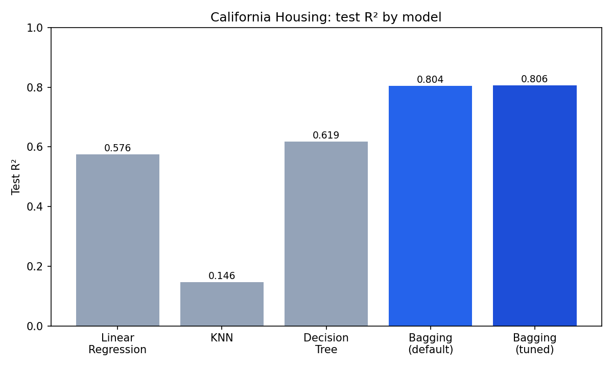

Linear regression and the lone decision tree land in the same neighbourhood (0.576 and 0.619), unsurprising since a single tree here isn't deep enough relative to the data to overfit as badly as in the toy example above. The real surprise is KNN, which collapses to 0.146. That's not KNN being a bad algorithm, it's KNN on unscaled features: this dataset mixes median income (roughly 0 to 15), room counts (single digits to hundreds), and latitude/longitude (30s to -120s), and distance-based methods are dominated by whichever column happens to have the largest raw numbers. KNN needs its inputs standardized first; none of the other four models here do, which is exactly why the gap is this large.

With zero tuning, BaggingRegressor's default settings already reach 0.804, comfortably ahead of every single model. Its train score is 0.974, still overfitting some, but far less than the lone tree would if grown this deep on the full feature set, and the gap between train and test has shrunk enough that the test number is meaningfully better.

4. Tuning It

Same search-don't-guess advice as Ch.46, now with GridSearchCV:

from sklearn.model_selection import GridSearchCV
 
param_grid = {
    "n_estimators": [50, 100, 300],
    "max_samples": [0.5, 1.0],
    "max_features": [0.5, 1.0],
    "bootstrap": [True, False],
    "bootstrap_features": [True, False],
}
search = GridSearchCV(
    BaggingRegressor(estimator=DecisionTreeRegressor(random_state=42), n_jobs=-1),
    param_grid=param_grid, cv=3, scoring="r2", n_jobs=-1,
).fit(X_train, y_train)
 
# best_params_: {'bootstrap': True, 'bootstrap_features': False,
#                'max_features': 1.0, 'max_samples': 1.0, 'n_estimators': 300}
# best_score_ (CV): 0.802

The search's own cross-validated score (0.802) lands almost exactly where the untuned default already was (0.804 on the held-out set), and the tuned model's actual test score, 0.806, is barely different. On this particular dataset the default bagging configuration was already close to as good as a grid search over 72 combinations gets you. That's a useful thing to know, not every dataset rewards heavy tuning, but it's also exactly why you run the search rather than assume it up front: the video's own numbers on load_boston showed a bigger jump (default test R² 0.81 to a tuned cross-validated score around 0.878), so how much tuning buys you is dataset-dependent, not a fixed rule of thumb.

5. What to Take Away

• BaggingRegressor is BaggingClassifier with a different last step: mean instead of majority vote. Every hyperparameter, every variant (bagging, pasting, random subspaces, random patches), carries over unchanged.
• A single fully-grown tree can hit a perfect training fit and still lose on test data; bagging trades away some of that training fit for a large gain in test performance, the bias-variance tradeoff made visible.
• Distance-based models like KNN need scaled features to be evaluated fairly against models like decision trees and bagging that don't care about feature scale.
• Tune with GridSearchCV or RandomizedSearchCV, not by hand, but don't assume the search will always move the needle far: sometimes the untuned default is already close to as good as it gets.

Next: Random Forest, bagging-of-trees with feature sampling moved inside each split instead of applied per tree.