Ch.46: The Bagging Classifier in Code

Inspired by: YouTube

Ch.45 built the intuition for bagging: train one algorithm many times on different random subsets of the data, then vote. This is the code half for classification, BaggingClassifier.

There is no companion notebook for this video in the course's usual repo, so every number and chart below comes from running scikit-learn fresh.

1. One Tree Overfits, 500 Don't

Start with the problem bagging solves. A fully grown decision tree on a noisy 2-D set memorises the training data (100% train accuracy) and draws a boundary full of thin rectangular fingers reaching out to individual points. Wrap 500 of those trees in a BaggingClassifier, each fit on a random quarter of the rows, and the voted boundary is smooth:

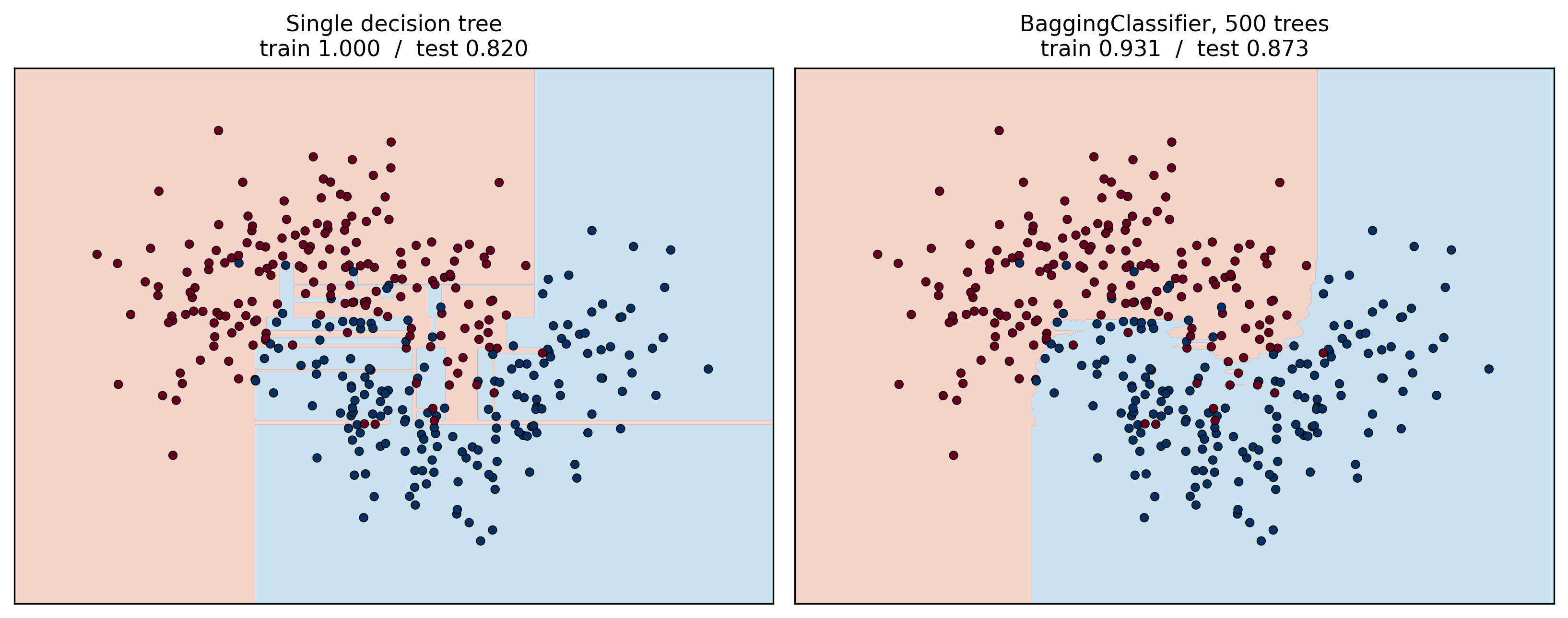
The single tree's train/test gap is 1.000 vs 0.820, a classic overfit. Bagging closes most of it: train drops to 0.931 (it no longer memorises), test rises to 0.873. The variance the single tree had is being averaged away.

2. BaggingClassifier in scikit-learn

from sklearn.datasets import make_classification
from sklearn.ensemble import BaggingClassifier
from sklearn.tree import DecisionTreeClassifier
from sklearn.model_selection import train_test_split
 
X, y = make_classification(
    n_samples=10_000, n_features=20, n_informative=8,
    n_redundant=4, flip_y=0.05, class_sep=0.8, random_state=42,
)
X_tr, X_te, y_tr, y_te = train_test_split(X, y, test_size=0.2, random_state=42)
 
bag = BaggingClassifier(
    estimator=DecisionTreeClassifier(),  # the base model, fully grown
    n_estimators=500,                    # how many of them
    max_samples=0.25,                    # rows each one gets: 0.25 => 25% of the training set
    bootstrap=True,                      # draw those rows WITH replacement
    random_state=42,
    n_jobs=-1,                           # train the trees in parallel
)
bag.fit(X_tr, y_tr)

The knobs that matter:

• estimator: the base model. Defaults to a decision tree; that's almost always what you want, because trees are the high-variance model bagging is built for.
• n_estimators: number of base models. More is better up to a plateau, then it's just compute (Ch.45's chart).
• max_samples: rows per base model, as a fraction (0.25) or an absolute count (2500). This is the main tuning knob.
• bootstrap: True samples rows with replacement (bagging), False without (pasting).

bag.estimators_samples_ is a list of the row indices each tree was trained on, one array per tree, useful for confirming each tree really did get its own slice.

3. The Four Variants Are Four Settings

Ch.45's table of bagging / pasting / random subspaces / random patches isn't four classes, it's four combinations of the row and column knobs on this one class:

# Pasting: rows without replacement
BaggingClassifier(estimator=DecisionTreeClassifier(), n_estimators=300,
                  max_samples=0.25, bootstrap=False)
 
# Random Subspaces: all rows, a random half of the columns per tree
BaggingClassifier(estimator=DecisionTreeClassifier(), n_estimators=300,
                  max_samples=1.0, bootstrap=False,
                  max_features=0.5, bootstrap_features=True)
 
# Random Patches: sample both
BaggingClassifier(estimator=DecisionTreeClassifier(), n_estimators=300,
                  max_samples=0.25, bootstrap=True,
                  max_features=0.5, bootstrap_features=True)

10-fold CV accuracy on the 10k-row, 20-feature set above:

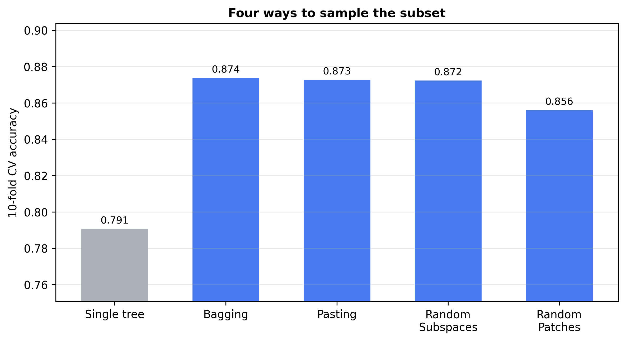
Any of the four turns a single tree's 0.791 into roughly 0.87, an eight-point jump. Between the four the differences are small: bagging edges it here, random patches trails slightly. The video's advice matches: bagging is the usual best default, but the gap is small enough that you should try all of them. Random subspaces and random patches earn their place mainly on high-dimensional data (images, text), where column diversity does more than row diversity.

You can flip through all four in the Ch.45 explorer with the "Row sampling" and "Features per tree" toggles.

4. Bagging an SVM Barely Helps

estimator doesn't have to be a tree, but the choice isn't free:

from sklearn.svm import SVC
 
BaggingClassifier(estimator=SVC(kernel="rbf", C=1), n_estimators=50,
                  max_samples=0.25, bootstrap=True, n_jobs=-1)

An RBF SVM is already a low-variance model: its boundary doesn't swing much when the training data changes. Bagging removes variance, so applied to a model that has little, it does almost nothing, and can cost you a little from training each SVM on only a quarter of the data. Single SVM here scores 0.884 on the held-out set; the 50-model bag scores 0.866, slightly worse. Bagging pays off in proportion to how much variance the base model has, which is why trees are the canonical choice.

5. The Out-of-Bag Score: Free Validation

When you sample rows with replacement, some rows get drawn multiple times for a given tree and some are never drawn at all. Statistically, each tree's bootstrap sample covers about 63% of the unique training rows (with max_samples=1.0), leaving roughly 37% "out of bag" for that tree, rows it never saw during training.

Those out-of-bag rows are a ready-made validation set: for each training row, average the predictions of only the trees that didn't train on it, and compare to the truth. That's the out-of-bag score, and it comes for free, no separate hold-out needed:

bag = BaggingClassifier(
    estimator=DecisionTreeClassifier(), n_estimators=500,
    max_samples=0.25, bootstrap=True, oob_score=True,  # <-- turn it on
).fit(X_tr, y_tr)
 
bag.oob_score_          # ~0.87, computed on rows each tree never trained on
bag.score(X_te, y_te)   # ~0.87 on the real hold-out, close to it

It really does track the held-out number:

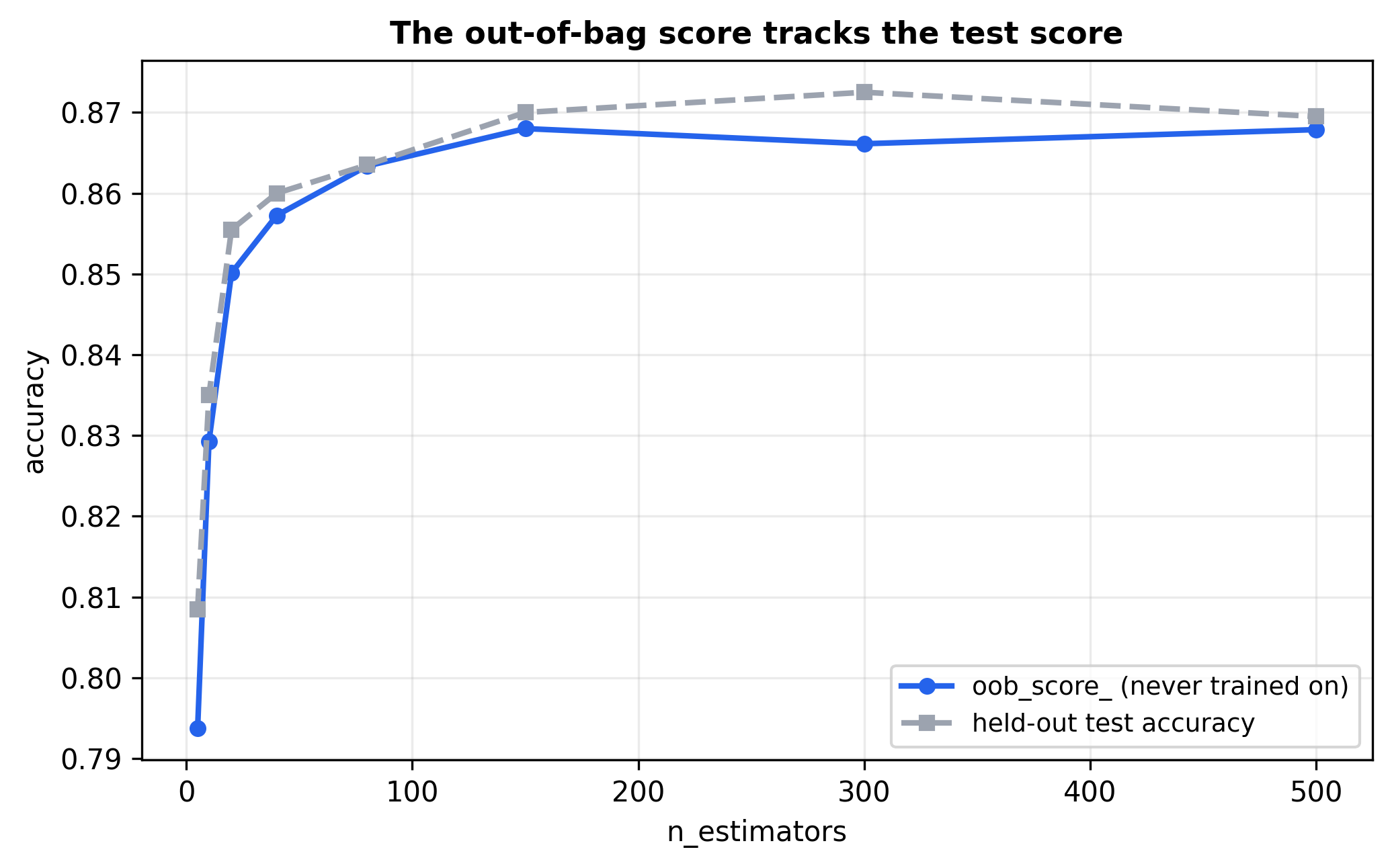
The out-of-bag score sits within about half a point of the true test accuracy across the whole range. On a small dataset where you'd rather not spend rows on a validation split, oob_score=True is close to a free lunch. (It needs bootstrap=True; pasting has no out-of-bag rows to speak of.)

6. Tuning It

There are four or five interacting knobs and no reliable way to guess them, so search. RandomizedSearchCV over a sensible grid is the practical choice:

from sklearn.model_selection import RandomizedSearchCV
 
param_dist = {
    "n_estimators": [50, 100, 300, 500],
    "max_samples": [0.1, 0.25, 0.4, 0.5, 0.7, 1.0],
    "bootstrap": [True, False],
    "max_features": [0.5, 0.7, 1.0],
    "bootstrap_features": [True, False],
}
search = RandomizedSearchCV(
    BaggingClassifier(estimator=DecisionTreeClassifier(), n_jobs=-1),
    param_distributions=param_dist, n_iter=25, cv=5,
    scoring="accuracy", random_state=42,
).fit(X_tr, y_tr)
 
# best_params_: {'n_estimators': 100, 'max_samples': 1.0, 'bootstrap': False,
#               'max_features': 0.5, 'bootstrap_features': False}
# best_score_ : 0.880

On this data the search landed on no row sampling (max_samples=1.0, bootstrap=False) with half the columns per tree, essentially random subspaces, and only edged the fixed bagging config from Section 3 (0.874 to 0.880). Which knobs win is data-dependent; that's the whole reason to search.

The practical takeaways from the video's own experiments:

• Bagging usually beats pasting, but the margin is small; try both.
• For row sampling, max_samples in the 0.25 to 0.5 range is a good starting point (though the search above preferred 1.0 here).
• Reach for feature sampling (random subspaces / patches) when the column count is large.
• Don't hand-pick the four knobs. Run GridSearchCV or RandomizedSearchCV.

7. What to Take Away

• BaggingClassifier(estimator=..., n_estimators=..., max_samples=..., bootstrap=...). Vote of many high-variance trees, each on its own row subset.
• Bagging / pasting / random subspaces / random patches are bootstrap × max_features × bootstrap_features settings of that one class, not separate algorithms. All four beat a single tree by a lot; the gaps between them are small.
• Bagging helps in proportion to the base model's variance: big win for trees, near-nothing for an SVM or linear model.
• oob_score=True gives a validation estimate for free from the ~37% of rows each tree never trains on, and it tracks the real test score closely.
• Four-plus interacting knobs means you tune with a search, not by hand.

Next: the bagging regressor in code, then Random Forest, which is bagging-of-trees with feature sampling moved inside each split.