
Ch.44: The Voting Regressor in Code
Inspired by: YouTube
Ch.42 built the case for voting, and Ch.43 built it in code for classification. This one is the regression half: VotingRegressor, which is simpler than its classifier counterpart, there's no hard/soft distinction to make, only one way to combine predictions.
No matching notebook exists in the course's usual companion repo for this video, and the video's own dataset (load_boston) has since been removed from scikit-learn over fair-housing concerns baked into the data, so every number and chart below comes from running the code fresh on the California housing dataset instead.
1. There's Only One Kind of Vote
A classifier votes on a discrete label, hence hard vs soft. A regressor's base models each already output a single real number, so there's nothing to choose between, VotingRegressor just averages them:
where is the -th base model's prediction and the number of base models. That's the entire mechanism. Everything else in this post, weights, hyperparameter diversity, is the same machinery as the classifier version, just applied to an average instead of a vote count.
2. Try It: Three Models, One Line
Pick a toy 1-D dataset and toggle which base models are in the vote. Each dashed line is one model fit on its own; the solid blue line is their average, the voting regressor's actual prediction.
Dashed lines are each base model on its own; the solid blue line is their averaged prediction, the voting regressor.
Worth actually testing, not just reading:
- On Linear (Noisy), all three models land close to the same line, there's nothing for voting to fix, so the ensemble's R² barely differs from the best individual model.
- On Sine Wave, Linear Regression can only draw a straight line through a curve, it's the clear weak link. Averaging it in still pulls the vote away from the curve that SVR and the tree trace far better on their own. This is the regression mirror of Ch.42's warning: a bad-enough base model drags the average down, it doesn't get outvoted the way a single bad classifier can.
- On Outlier, watch the tree gap around the three flung-out points (it can carve them into their own leaf) while SVR and linear regression get bent by them to different degrees. The vote lands between all three reactions.
- On Step, none of these three models is built to draw a clean corner, linear regression can't bend, SVR smooths across it, only the tree gets close by nature, but its single split still isn't sharp until it's deep enough. Watch how far the voted average sits from the actual step.
(The explorer's three estimators are compact from-scratch implementations, not the sklearn versions, tuned to show qualitatively similar curves. The rest of this post uses real sklearn code on a real dataset.)
3. VotingRegressor in scikit-learn
from sklearn.datasets import fetch_california_housing
from sklearn.linear_model import LinearRegression
from sklearn.svm import SVR
from sklearn.tree import DecisionTreeRegressor
from sklearn.ensemble import VotingRegressor
from sklearn.model_selection import cross_val_score
from sklearn.preprocessing import StandardScaler

data = fetch_california_housing()
X, y = data.data, data.target  # 20,640 rows, 8 columns, target = median house value

X = StandardScaler().fit_transform(X)

lr = LinearRegression()
svr = SVR(kernel="rbf", C=5)
tree = DecisionTreeRegressor(max_depth=6, random_state=42)

estimators = [("lr", lr), ("svr", svr), ("tree", tree)]
vote = VotingRegressor(estimators=estimators)
Same (name, estimator) list convention as VotingClassifier. cross_val_score treats vote like any other regressor:
for name, model in estimators + [("voting", vote)]:
    print(name, cross_val_score(model, X, y, cv=10, scoring="r2").mean())
Run on a 3,000-row sample of California housing (full-size SVR training is slow enough that a sample keeps this reproducible without a coffee break), 10-fold CV R²:
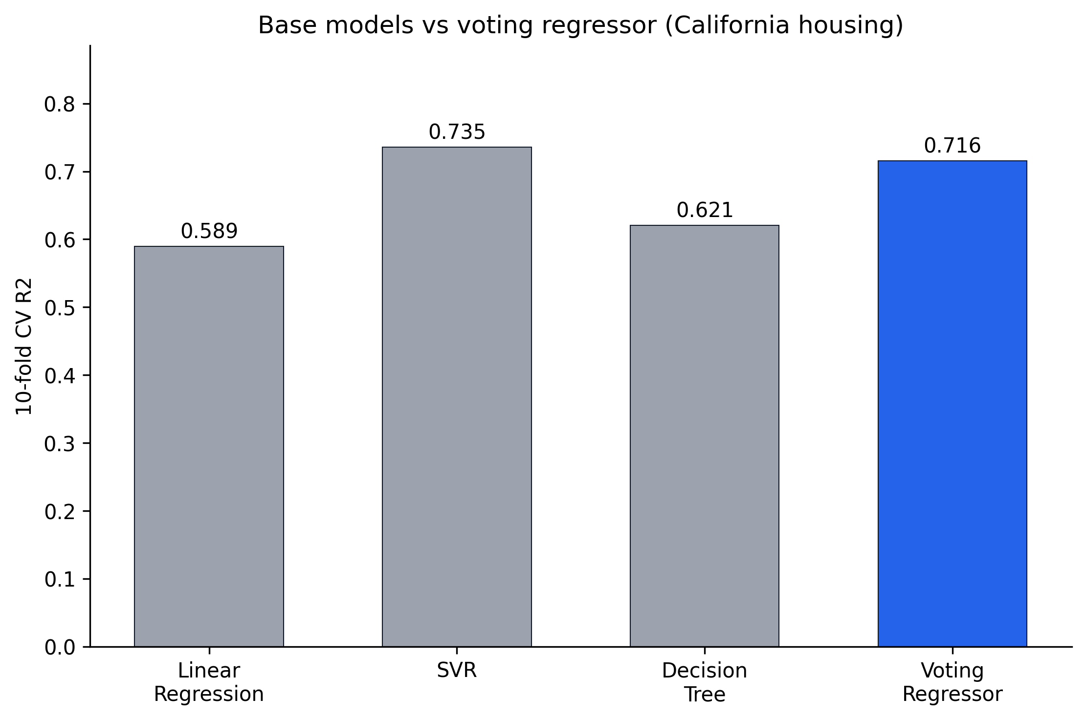
The voting regressor (0.716) beats two of its three base models comfortably but falls just short of the best one, SVR alone at 0.736. That's expected, not a bug: SVR is the strongest model here by a wide margin, and averaging its prediction with two weaker ones pulls the result toward the middle. Voting helps most when the base models are close in skill; when one is clearly better than the rest, plain averaging can leave you worse off than just using the winner. That's exactly the problem weights exist to fix.
4. Weights: Give the Stronger Model More Say
VotingRegressor takes the same weights argument as VotingClassifier, changing the average from a plain mean to a weighted one:
VotingRegressor(estimators=estimators, weights=[1, 3, 1])Random Forest's probability got upweighted in the classifier post; here it's SVR's turn, since it's the strongest of the three on this data. Brute-force search confirms the instinct:
from itertools import product

best = None
for w1, w2, w3 in product(range(1, 4), repeat=3):
    vr = VotingRegressor(estimators=estimators, weights=[w1, w2, w3])
    score = cross_val_score(vr, X, y, cv=5, scoring="r2").mean()
    if best is None or score > best[1]:
        best = ((w1, w2, w3), score)
Top of the full 27-combination grid over weights=[w1, w2, w3] for w1, w2, w3 in 1..3, base scores lr=0.591, svr=0.732, tree=0.597:
| Weights (lr, svr, tree) | CV R² |
|---|---|
| (1, 3, 1) | 0.732 |
| (1, 3, 2) | 0.726 |
| (1, 2, 1) | 0.725 |
| (2, 3, 1) | 0.721 |
| equal (1, 1, 1) | 0.709 |
Weighting SVR three times as heavily as the other two (0.732) nearly matches SVR's own solo score (0.732) while still keeping the other two models in the mix as a hedge, and it clears equal weighting (0.709) by 2.3 points. The pattern from Ch.43 holds exactly: weight by how much you trust each model, then search rather than guess the precise numbers.
5. Diversity Without Different Algorithms
Same second route as the classifier post: take one algorithm, fit it several times at different hyperparameter values, and vote across those instead of across different algorithms.
max_depth for a decision tree is a good candidate, there's rarely a principled way to know the right depth upfront without trying several:
depths = [2, 4, 6, 8, 12]
tree_estimators = [
    (f"tree_d{d}", DecisionTreeRegressor(max_depth=d, random_state=42))
    for d in depths
]
vote = VotingRegressor(estimators=tree_estimators)
Held-out test R² per depth, plus the vote across all five:
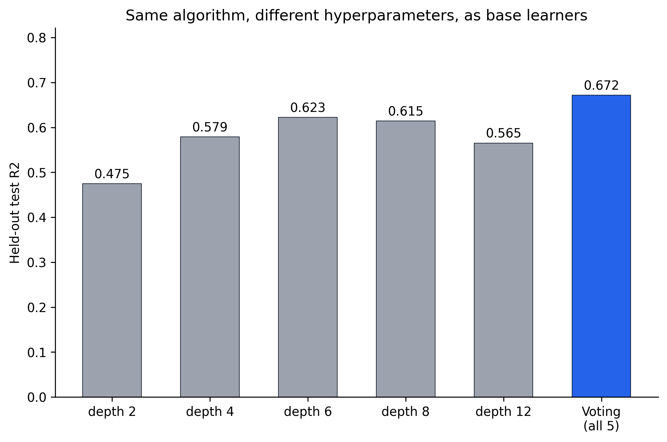
Here voting does better than the single best hyperparameter, not just better than average: depth 6 alone tops out at 0.623, but voting across all five reaches 0.672. This is the opposite outcome from Ch.43's SVM-degree example, where voting landed between the best and the average. The difference is what each individual tree gets wrong: shallow trees underfit smooth regions while deep trees overfit noisy ones, and averaging five different depths cancels a good chunk of each one's particular mistake, closer to genuinely independent errors than five SVMs at different polynomial degrees turned out to be. Whether hyperparameter-diversity voting beats the single best setting isn't guaranteed either way, it depends on how differently each setting fails, which is itself something you only find out by trying.
6. What to Take Away
VotingRegressor(estimators=[...]). No hard/soft choice, it always averages the base models' raw predictions.- Voting doesn't reliably beat the single strongest base model when that model is far ahead of the rest, it pulls the average toward the middle instead.
weightsfixes exactly that: give the stronger model more say, search for the actual numbers rather than assume.- The same hyperparameter-diversity trick from Ch.43 applies here too, and here it actually beat the best single setting, a reminder that whether that trade pays off depends on the data, not a rule you can apply blind.
Next up: ensemble families that build their own diversity instead of relying on you to supply it, starting with bagging.