Ch.42: Voting Ensembles, the Intuition and the Proof

By Ayush Arora•2026-09-04•8 min read

Inspired by: YouTube

Voting is the first and simplest of the four ensemble families from the previous post. It gets three posts: this one is pure intuition and the probability argument for why voting works, the next one builds a voting classifier in code, and the one after that does a voting regressor. No companion notebook here; the charts below are computed from the same arithmetic the video works by hand.

1. The Setup

Take a handful of models, say three, and call them the base learners:

Model 1, Model 2, Model 3.

Each one is trained independently on the training data. The base learners can be three different algorithms (a KNN, a logistic regression, a decision tree), or three copies of the same algorithm; both cases show up in the next post. What matters for now is that they are trained separately and there is no communication between them.

To predict on a new point, hand it to all three and combine their answers:

Classification: take the majority vote. If two or more models say class 1, the ensemble says class 1.
Regression: take the mean. Add the three predicted numbers and divide by three.

That is the whole algorithm. It is democracy: everyone gets one equal vote, and the group decision is whatever most members picked.

2. Two Conditions the Base Models Must Meet

Voting does not always help. It helps only when two things hold.

1. The base models must be as independent as possible. If all three models make the same mistakes on the same rows, pooling their votes changes nothing; you have one model asked three times. The value comes from the models being wrong in different places, so that where one slips, the other two can outvote it. This is why voting ensembles pair up different algorithms: different assumptions lead to different errors.

2. Every base model must be better than random guessing. For binary classification that means accuracy above 50%. If the base models are worse than a coin flip, voting does not just fail to help, it actively hurts: the ensemble ends up worse than the worst individual model. Section 5 shows this happening.

The KBC "ask the audience" analogy from the last post is the intuition for condition 1. A room full of computer-science people is a great crowd for a programming question and a useless one for anything outside that domain, because their knowledge is correlated. A room with a chartered accountant, an engineer, a doctor, a painter, and a poet covers more ground: whatever the question, someone in the mix probably knows, and the rest do not all fail together.

3. Why It Works, as Probability

Here is the part that feels like it should not be true. Suppose you have three models, each with 70% accuracy. How can majority-voting them produce something more accurate than 70%, better than every model that went into it?

Set it up carefully. The three models are independent, and each is correct on a random new point with probability 0.7 and wrong with probability 0.3. Independence means the probability of any specific combination of right/wrong across the three is just the product of the individual probabilities.

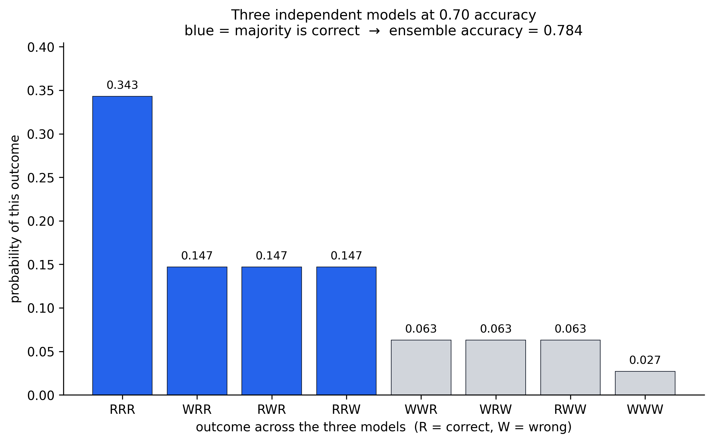
There are eight possible outcomes. Writing R for "correct" and W for "wrong", ordered as (Model 1, Model 2, Model 3):

Outcome	Probability	Majority vote
R R R	0.7 × 0.7 × 0.7 = 0.343	correct
R R W	0.7 × 0.7 × 0.3 = 0.147	correct
R W R	0.7 × 0.3 × 0.7 = 0.147	correct
W R R	0.3 × 0.7 × 0.7 = 0.147	correct
R W W	0.7 × 0.3 × 0.3 = 0.063	wrong
W R W	0.3 × 0.7 × 0.3 = 0.063	wrong
W W R	0.3 × 0.3 × 0.7 = 0.063	wrong
W W W	0.3 × 0.3 × 0.3 = 0.027	wrong

The eight probabilities add to 1, as they must.

The ensemble is correct exactly when at least two of the three models are correct: the top four rows. Add them:

0.343 + 0.147 + 0.147 + 0.147 = 0.784

The voting ensemble is right 78.4% of the time. Three 70% models, combined by a plain majority vote, give you a 78% model. The gain is real and it comes entirely from the independence assumption: the cases where one model slips but the other two hold (the three 0.147 rows) get rescued by the vote.

Bar chart of the eight right/wrong outcomes for three independent models at 0.70 accuracy, sorted by probability. The RRR bar is 0.343, the three bars with two correct are each 0.147, the three bars with one correct are each 0.063, and WWW is 0.027. The four bars where the majority is correct (RRR and the three two-correct bars) are coloured blue and labelled as summing to an ensemble accuracy of 0.784

4. Generalising: the Condorcet Curve

The 70% example is one point on a curve. For an odd number $n$ of independent models, each correct with probability $p$ , the majority vote is correct with probability

P_\text{vote} = \sum_{k > n/2} \binom{n}{k}\, p^k (1-p)^{n-k}

Plot that against $p$ for a few values of $n$ :

Line chart with individual base model accuracy p on the x-axis from 0 to 1 and majority-vote accuracy on the y-axis. A dashed diagonal marks the single-model baseline. Four S-shaped curves for majority votes of 3, 11, 51 and 201 models all pass through the point (0.5, 0.5). To the right of 0.5 they bow above the diagonal and steepen toward 1 as n grows; to the left of 0.5 they bow below the diagonal and drop toward 0. Two red dots mark the video's hand-worked points: 0.70 maps to 0.784 and 0.30 maps to 0.216 on the n equals 3 curve

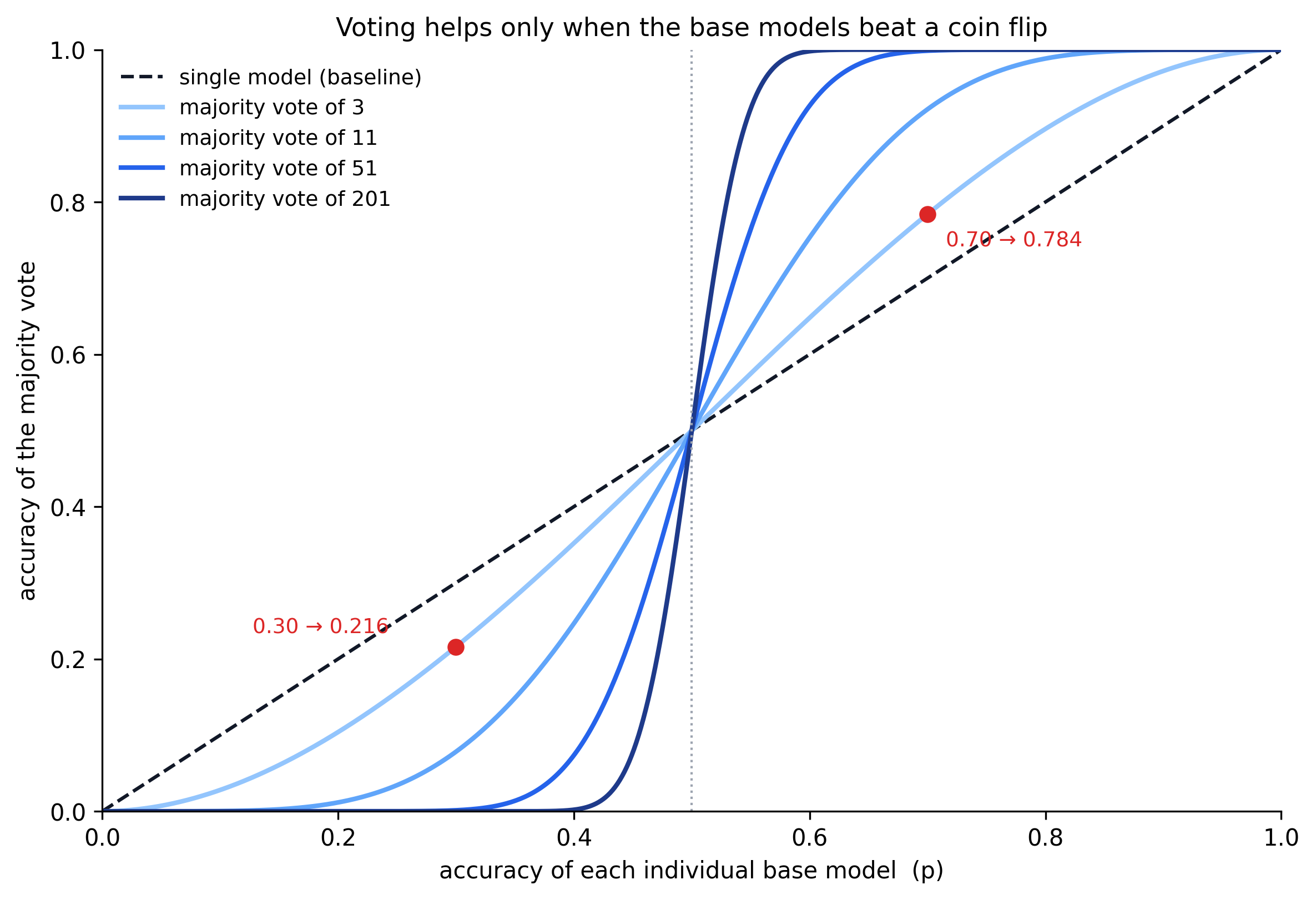
Everything about voting is in this picture:

All curves cross at $p = 0.5$ . Voting a pile of coin flips gives you a coin flip. No amount of aggregation manufactures signal that is not there.
To the right of 0.5, the curve sits above the diagonal. Base models better than random combine into something better than any of them, and the effect strengthens as $n$ grows. With enough independent 60% models the vote approaches 100%.
To the left of 0.5, the curve sits below the diagonal. This is condition 2 failing, and it is the subject of the next section.

5. The Mirror Case: When Voting Backfires

Run the same enumeration with three independent models at 30% accuracy each. Now $p = 0.3$ , $1 - p = 0.7$ , and the ensemble is still correct when at least two of three are correct:

\underbrace{0.3^3}_{\text{all three}} + \underbrace{3 \times (0.3 \times 0.3 \times 0.7)}_{\text{exactly two}} = 0.027 + 0.189 = 0.216

The voting ensemble is right 21.6% of the time, worse than each 30% model that went into it. When the base models are more often wrong than right, the majority vote amplifies the wrongness: the outcomes where two of three models fail together now dominate, and the vote follows them off the cliff.

This is the concrete reason for condition 2. A voting ensemble is not a safety net you can throw over anything. Feed it models that lose to a coin flip and it makes them worse. In practice this is a low bar, since almost any real trained model clears 50% on a binary problem, but it is worth knowing the failure mode exists and is not gentle.

6. What to Take Away

Voting: train several models independently on the same data, then majority-vote (classification) or average (regression) their predictions.
It works because independent errors get outvoted. The more the base models disagree, the more the ensemble gains.
It needs base models that each beat random guessing. Below that line, voting hurts.
Three 70% models becoming a 78% model is not a trick; it is just the probability of "at least two of three independent events" working in your favour.

The next post puts this to work: a VotingClassifier in scikit-learn, comparing hard voting against soft voting, and checking whether the real-world numbers line up with the arithmetic here.

View all chapters in Machine Learning Algorithms →