
Ch.43: The Voting Classifier in Code
Inspired by: YouTube
Last post worked out why voting helps, three independent 70%-accurate models becoming a 78.4%-accurate ensemble. This one builds the thing: scikit-learn's VotingClassifier, the hard/soft distinction, weights, and a second way to get diverse base models that doesn't require different algorithms at all.
No matching notebook exists in the course's usual companion repo for this video, so every number and chart below comes from running the code fresh rather than copying figures off a whiteboard.
1. Hard Voting vs Soft Voting
VotingClassifier takes a list of (name, estimator) pairs and a voting argument. That argument is the whole distinction:
voting="hard": each base model outputs a class label. The ensemble's prediction is whichever label got the most votes. This is exactly the majority vote from the last post.voting="soft": each base model outputs a probability for each class (predict_proba). The ensemble averages those probabilities across models, then predicts whichever class has the higher average.
Concretely, for a binary problem with three base models predicting P(class 1) = 0.2, 0.8, 0.6:
- Hard voting only sees the labels each of those imply (
0, 1, 1), so it votes class 1, 2 votes to 1. - Soft voting averages the probabilities:
(0.2 + 0.8 + 0.6) / 3 = 0.53, still class 1, but as a much closer call. If the third model had said0.35instead of0.6, hard voting would still land on class 1 (labels0, 1, 0→ wait, that's a tie broken by the first-listed model in practice, but the point holds) while soft voting's average0.45flips to class 0. Soft voting is sensitive to how confident each model is, not just which side of 0.5 it landed on. That extra information is usually worth having, which is why soft voting tends to outperform hard voting, though not always.
Every base estimator used in soft voting must implement predict_proba. LogisticRegression, KNeighborsClassifier, and tree ensembles all do; a plain SVC needs probability=True (which internally fits an extra calibration step, so it's slower to train).
2. Try It: Six Datasets, Five Estimators
Pick a dataset shape, pick two to four base estimators, and switch between hard and soft voting. The main panel is the combined ensemble's decision boundary; the strip underneath shows each base model on its own, with its individual accuracy.
Hard voting: each model casts one class vote, the region colour follows the majority.
A few things worth actually testing here, not just reading:
- On XOR and Two Spirals, Logistic Regression alone is close to useless (it can only draw a straight line), but adding it to a vote with SVM or Random Forest costs the ensemble almost nothing, since the other members outvote its mistakes. This is condition 1 from the last post: independent errors get outvoted.
- On Outlier, watch what a single mislabelled/far-flung point does to each model's boundary individually versus what it does to the vote. KNN and the tree-based models bend hard around it; Logistic Regression barely notices; the ensemble sits in between.
- Switch Concentric Circles between hard and soft voting with Logistic Regression included. Its boundary is a straight line no matter what, so it's confidently wrong across roughly half the circle. Under soft voting that confident wrongness pulls the averaged probability further than a single vote would under hard voting, exactly the "soft voting is sensitive to confidence" point above, and here it's sensitive in the wrong direction.
(The explorer's five estimators are compact from-scratch implementations, not the sklearn versions, tuned to show qualitatively similar decision boundaries. The rest of this post uses real sklearn code, and the plots below are computed from actual cross_val_score and train/test runs.)
3. VotingClassifier in scikit-learn
from sklearn.linear_model import LogisticRegression
from sklearn.neighbors import KNeighborsClassifier
from sklearn.ensemble import RandomForestClassifier, VotingClassifier
from sklearn.model_selection import cross_val_score

lr = LogisticRegression(max_iter=1000)
knn = KNeighborsClassifier()
rf = RandomForestClassifier(n_estimators=100, random_state=42)

estimators = [("lr", lr), ("knn", knn), ("rf", rf)]

hard_vote = VotingClassifier(estimators=estimators, voting="hard")
soft_vote = VotingClassifier(estimators=estimators, voting="soft")
estimators is a list of (name, model) tuples, not just a list of models, the same convention Pipeline uses. cross_val_score treats hard_vote and soft_vote like any other estimator:
for name, model in estimators + [("hard voting", hard_vote), ("soft voting", soft_vote)]:
    print(name, cross_val_score(model, X, y, cv=10).mean())
Run on a moderately hard synthetic binary dataset (12 features, meaningful class overlap, make_classification(class_sep=0.6)), the three base models land well apart in skill, and voting sits above the pack:
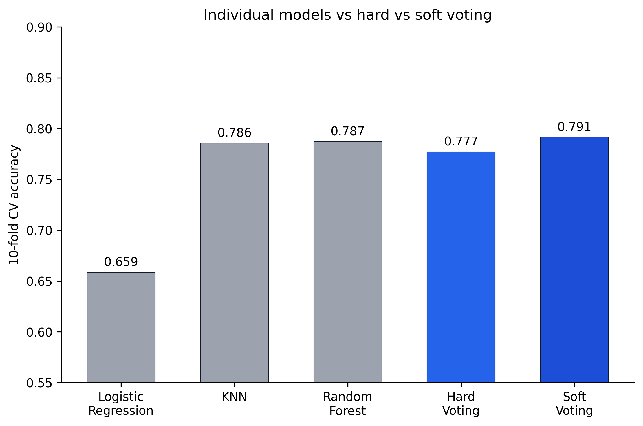
Soft voting (0.791) edges out every individual model, including the best one (Random Forest at 0.787). Hard voting (0.777) actually falls below the best individual model here, a reminder that this is a real dataset with real correlated errors, not the idealised independent-70%-models arithmetic from the last post. Logistic Regression drags the hard vote down by throwing a full vote at every prediction even when it is barely better than a coin flip on this data; soft voting lets its low-confidence votes matter less.
The video makes the same point on real data it deliberately made hard: keep only Iris's virginica/versicolor rows (dropping setosa, which every model separates trivially) and only sepal length/sepal width as features, two classes that overlap heavily on just those two columns. Reproducing that setup, LogisticRegression alone reaches ≈0.75 10-fold CV accuracy, comfortably ahead of KNeighborsClassifier (≈0.59) and RandomForestClassifier (≈0.60) on this particular subset. Voting the three together under voting="hard" lands at ≈0.66, worse than just using Logistic Regression by itself. This is the case the video is careful to call out: a voting ensemble is not automatically the right choice, sometimes the honest answer is to check the individual scores first and go with whichever single model is already winning.
4. Weights: Not Every Vote Has to Count the Same
By default every base model gets one equal vote. VotingClassifier accepts a weights argument to change that:
VotingClassifier(estimators=estimators, voting="soft", weights=[1, 2, 3])This means Random Forest's probability counts three times as much as Logistic Regression's when the votes are averaged. It is a hyperparameter like any other, searchable by brute force:
from itertools import product

best = None
for w1, w2, w3 in product(range(1, 4), repeat=3):
    vc = VotingClassifier(estimators=estimators, voting="soft", weights=[w1, w2, w3])
    score = cross_val_score(vc, X, y, cv=5).mean()
    if best is None or score > best[1]:
        best = ((w1, w2, w3), score)
Run on a second synthetic dataset where the base models are more spread out in skill (lr at 0.749, knn at 0.851, rf at 0.867 individually), the top of a full 27-combination grid search over weights=[w1, w2, w3] for w1, w2, w3 in 1..3:
| Weights (lr, knn, rf) | CV accuracy |
|---|---|
| (1, 2, 3) | 0.878 |
| (1, 3, 3) | 0.876 |
| (1, 2, 2) | 0.873 |
| (1, 3, 2) | 0.872 |
| equal (1, 1, 1) | 0.860 |
The best weighting (0.878) beats equal weighting (0.860) by almost 2 points, and it makes intuitive sense: it downweights the weakest model (lr) and upweights the strongest (rf), roughly in proportion to how each actually performs. That is the general pattern, weight base models by how much you trust them, though which exact combination wins is still something you search for rather than guess.
Weighting is also the fix for the Iris case from §3, where plain hard voting (≈0.66) lost to Logistic Regression alone (≈0.75). Sweeping weights=[i, j, k] for lr, knn, rf over i, j, k ∈ {1, 2, 3} (27 combinations, still hard voting), the best combination found is (3, 1, 1), three times the weight on lr and equal weight on the other two, which brings the ensemble back up to ≈0.75, matching Logistic Regression's own score rather than beating it. Heavily upweighting the model that was already winning doesn't manufacture a better ensemble here, it just stops the weaker models from dragging it down, which is exactly what happened without weights.
5. Diversity Without Different Algorithms
Everything so far pairs up different algorithms to get independent errors. There is a second route: take one algorithm, fit it several times with different hyperparameters, and vote across those instead.
This is useful specifically when a hyperparameter is hard to pick by eye. An SVM's degree (for a polynomial kernel) is a good example, there is often no principled way to guess it upfront:
from sklearn.svm import SVC

degrees = [1, 2, 3, 4, 5]
svm_estimators = [
    (f"svm_d{d}", SVC(kernel="poly", degree=d, probability=True))
    for d in degrees
]
vote = VotingClassifier(estimators=svm_estimators, voting="soft")
On a noisy two-moons dataset, held out test accuracy per degree, plus the vote across all five:
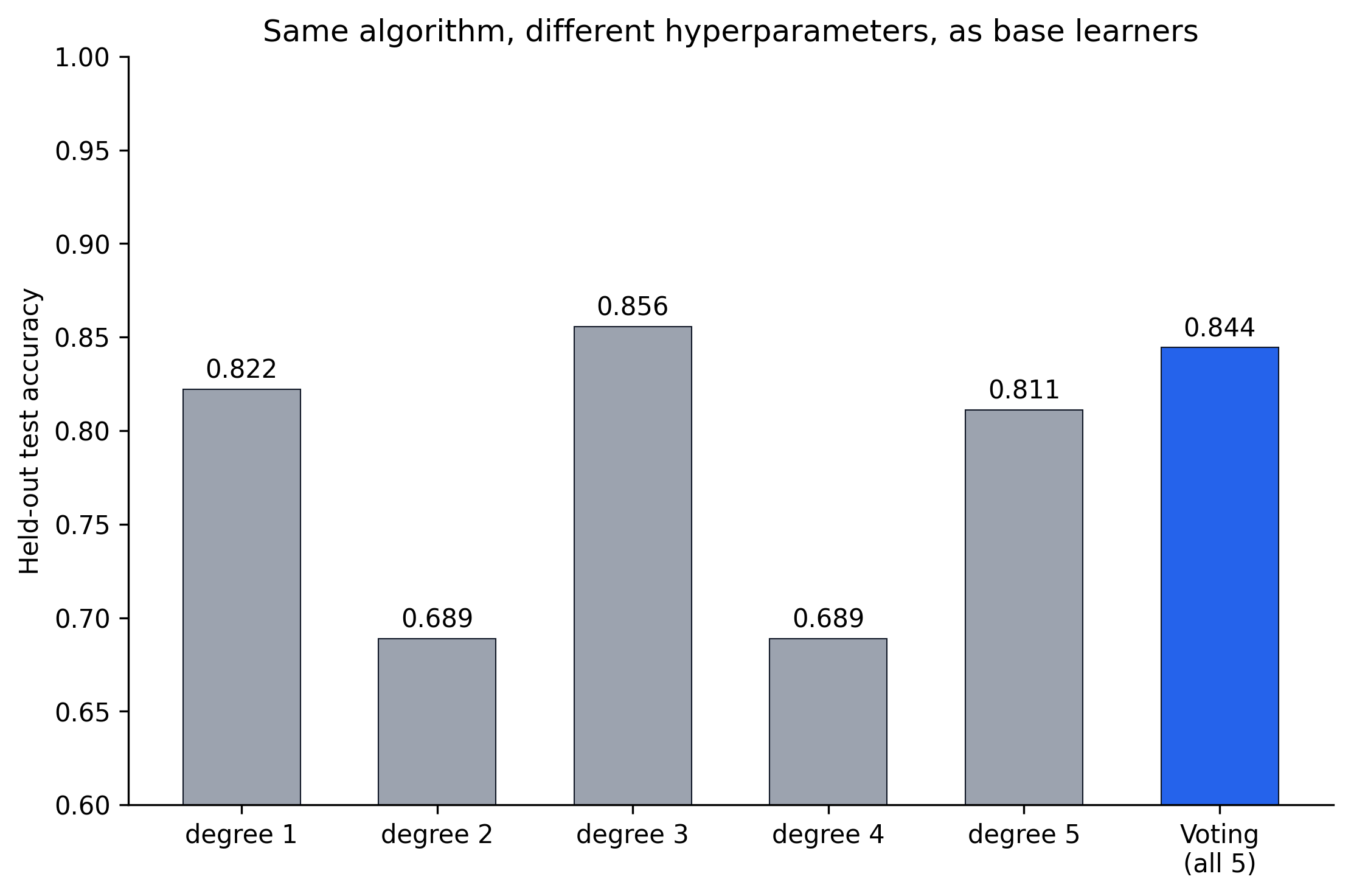
Two things stand out. First, degree matters a lot here, degree 3 (0.856) beats degree 2 (0.689) by 17 points, and you would not know which one to pick without trying them all. Second, the vote (0.844) doesn't beat the single best degree (0.856), but it comfortably beats the average degree and, crucially, it is nowhere near the worst ones (0.689). If you had picked degree 2 or 4 blind, you would have a much worse model; voting across all five is a way to never be that unlucky, at the cost of a small amount of the best-case upside. Whether that trade is worth it depends on whether you can afford a proper hyperparameter search (grid search or similar) instead, in which case that usually wins outright, or whether you want a reasonable answer without one.
6. What to Take Away
VotingClassifier(estimators=[...], voting="hard" | "soft"). Hard votes on labels, soft averages probabilities and is usually the better default when every base model supportspredict_proba.weightslets stronger base models count for more; there's no formula for the right weights, only search.- Diversity doesn't require different algorithms. The same algorithm at different hyperparameter settings works too, and is a decent hedge when you can't easily tell which setting is best.
- None of this is a guarantee. Ch.42 already showed the failure mode: base models worse than random make voting worse, not better. In the numbers above, hard voting even a set of good models underperformed the best individual one, because their errors weren't as independent as the clean-probability math assumes.
The next posts move to ensemble families that build their own diversity instead of relying on you to supply it: bagging and random forests.