Ch.3: What is a Perceptron? Perceptron vs Neuron and Geometric Intuition

By Ayush Arora•2026-10-04•15 min read

Inspired by: YouTube

The previous post wrapped up the theory. From here on we build things, and the right place to start is the perceptron, the fundamental building block of an artificial neural network.

It's worth being stubborn about this order. A multilayer perceptron is many perceptrons wired together, and training one is much easier to understand once you've seen how a single perceptron learns. Skipping straight to multilayer networks means learning two hard things at once.

The perceptron will take a few posts:

This post: what a perceptron is, how it predicts, how it compares to a biological neuron, its geometric intuition, and running it in code.
Next: how a perceptron is trained.
After that: the problem that limited the perceptron and made multilayer perceptrons necessary.

1. What a Perceptron Is

A perceptron is an algorithm for supervised machine learning, in the same family as linear regression, logistic regression or SVMs. What makes it special is its design: it happens to be shaped exactly right to serve as a building block for bigger networks.

Here is that design. Think of it as a mathematical function with a few parts:

A perceptron with two inputs: weighted sum, then activation.

Inputs ( $x_1$ , $x_2$ ): the feature values of one example, fed in from the left.
Weights ( $w_1$ , $w_2$ ): one per input, sitting on the connection between that input and the rest of the model.
Bias ( $b$ ): a weight on a connection whose input is always the constant 1. Its job becomes clear in the geometric section.
Summation: multiply each input by its weight, add everything up. This is a dot product plus the bias:

z = w_1 x_1 + w_2 x_2 + b

Activation function: takes $z$ and squeezes it into a fixed range. $z$ could be any number, since the inputs and weights could be anything, so the activation brings it into a range you can use as an output: $[0, 1]$ , $[-1, 1]$ , or something else depending on the function.

The perceptron uses the step function:

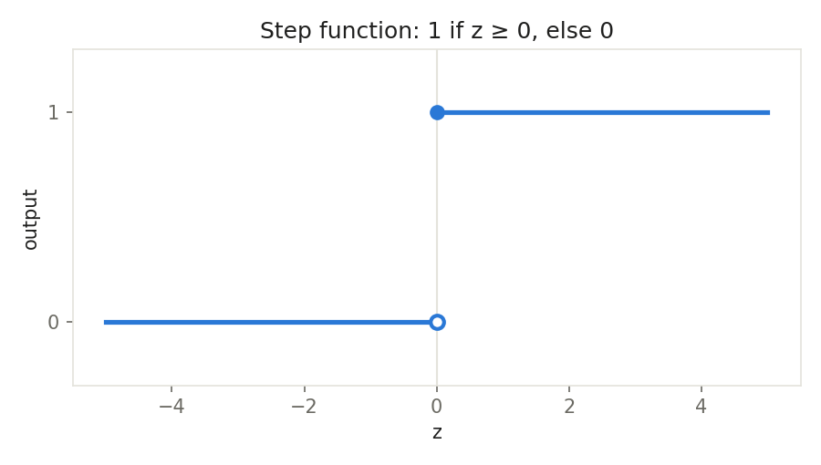
y = \begin{cases} 1 & \text{if } z \ge 0 \\ 0 & \text{if } z < 0 \end{cases}

Step function: output is 0 for all negative z, jumps to 1 at z equal to 0 and stays at 1 for all positive z

There are many other activation functions (ReLU and others you'll meet later in the series), but for now the step function is all we need. So the whole model is: inputs come in, get weighted and summed into $z$ , and $z$ passes through the step function to produce a 0 or a 1.

2. How a Perceptron Makes a Prediction

Take a concrete problem. You have data on 1000 students: each student's IQ, their college CGPA, and whether they got placed (1) or not (0). A couple of rows might look like:

IQ	CGPA	placed
78	7.8	1
69	5.1	0

You want a model that learns from this data and, given a new student's IQ and CGPA, predicts whether they'll get placed. Like any learning algorithm, the perceptron has two stages:

Training. Feed the students in one at a time: $x_1$ is the student's IQ, $x_2$ is their CGPA. You know the correct output for each one, so you can compare it with what the perceptron produces and adjust. The entire objective of training is to find good values for $w_1$ , $w_2$ and $b$ . How it does that is the next post.
Prediction. Once training has fixed the weights and bias, plug in a new student and read off the output.

Here's a prediction worked through. Suppose training gave $w_1 = 1$ , $w_2 = 2$ , $b = 3$ , and a new student has an IQ of 100 and a CGPA of 5.1:

z = 1 \cdot 100 + 2 \cdot 5.1 + 3 \cdot 1 = 100 + 10.2 + 3 = 113.2

$z \ge 0$ , so the step function outputs 1: the perceptron predicts this student will be placed. If $z$ had come out negative, the prediction would have been "not placed". That's all prediction is: a weighted sum and a threshold. Everything interesting lives in the values of the weights and bias.

More inputs? Suppose you add a third column, say which state the student is from. Add a third input $x_3$ with its own weight $w_3$ :

z = w_1 x_1 + w_2 x_2 + w_3 x_3 + b

Nothing else in the model changes. One input and one weight per column, however many columns there are.

3. Perceptron vs Biological Neuron

Deep learning is often described as inspired by the human nervous system. So how does a perceptron compare to a single biological neuron?

A nervous system is a collection of billions of neurons, the building blocks of the system. A neuron is a cell with three parts that matter here:

Dendrites, the root-like branches, where input arrives.
The nucleus, the cell body, where the internal processing happens.
The axon, the long thick fibre, which carries the output onward.

Put the two side by side and there is a rough correspondence:

Neuron	Perceptron
Dendrites (input)	Inputs and their weighted connections
Nucleus (processing)	Summation and activation
Axon (output)	The output $y$
Many neurons form a nervous system	Many perceptrons form a neural network

So the perceptron's inventor, Frank Rosenblatt, clearly took some inspiration from neurons. But saying a perceptron is a neuron, or is a faithful copy of one, is wrong. Three differences:

Complexity. A neuron is enormously complex: it can receive a huge number of inputs, and its output goes on to many other neurons. A perceptron is simple.
Internal processing. What happens inside a neuron's nucleus is a complex electrochemical process that still isn't fully understood. Inside a perceptron there are exactly two operations, a weighted sum and a step function, simple enough to plot.
Neuroplasticity. A neuron's connections change over time. They can grow thicker (a stronger connection) or thinner (a weaker one), disappear entirely, or new ones can form. This is how you pick up new skills. A perceptron's structure is fixed: the connections it starts with are the connections it keeps. Training does adjust the weights, which is a bit like connections strengthening or weakening, but that only happens in a separate training phase, and a perceptron can never grow a new connection or rewire itself.

The fair summary: the perceptron is weakly inspired by the neuron. The design borrows from it, but it isn't a copy.

4. Reading the Weights: Feature Importance

Back to the placement example. Suppose training gave $w_1 = 2$ (IQ), $w_2 = 4$ (CGPA) and $b = 1$ .

The weights tell you the strength of each connection: how much each input pushes $z$ up or down. Since CGPA's weight is twice IQ's, you might read this as "CGPA matters twice as much as IQ in deciding placement". That's the idea behind using a perceptron's weights as feature importance.

There's a catch, though. A weight measures the effect of one unit of its input, and one unit means very different things for different features. In this example IQ is around 100 while CGPA is between 0 and 10. With these weights, an IQ of 100 adds $2 \times 100 = 200$ to $z$ , while a CGPA of 8 adds only $4 \times 8 = 32$ . In practice IQ dominates the decision, even though its weight is smaller.

So comparing raw weights only works when the features are on the same scale. Standardize the inputs first (for example with scikit-learn's StandardScaler), retrain, and then compare weight sizes. The bias has an interpretation too, which comes up later.

5. Geometric Intuition

Seeing an algorithm work visually makes it much easier to understand. So let's look at what a perceptron does geometrically.

Written out in full, the perceptron is:

y = f(z), \quad z = w_1 x_1 + w_2 x_2 + b, \quad f(z) = \begin{cases} 1 & z \ge 0 \\ 0 & z < 0 \end{cases}

Plot the 1000 students on a scatter plot, IQ on one axis and CGPA on the other, with one colour for placed and another for not placed. Students with high IQ and high CGPA cluster together as placed; students with low values of both cluster as not placed. The goal is a predictor that takes a new point and says which group it belongs to.

Now look at the expression for $z$ and rename things: call $w_1$ " $A$ ", $w_2$ " $B$ ", $b$ " $C$ ", $x_1$ " $x$ " and $x_2$ " $y$ ". Then setting $z = 0$ gives

Ax + By + C = 0

which is the equation of a line. So a perceptron is, at heart, a line.

Then what are $Ax + By + C \ge 0$ and $Ax + By + C < 0$ ? They're not lines; they're regions: everything on one side of the line, and everything on the other side. The perceptron's rule says:

A point that lands in the $z \ge 0$ region is predicted placed (1).
A point that lands in the $z < 0$ region is predicted not placed (0).

That's the whole trick. The perceptron draws a line, the line divides the plane into two regions, and every point is classified by which region it falls in. Because it always produces exactly two regions, the perceptron is a binary classifier.

The parameters have clear geometric jobs too. The weights $w_1$ and $w_2$ set the line's tilt. The bias $b$ shifts the line without changing its tilt; without it, the line would be forced to pass through the origin.

More dimensions. Add a third input, say 12th-grade marks. Now each student is a point in 3D, and

w_1 x_1 + w_2 x_2 + w_3 x_3 + b = 0

is the equation of a plane. Picture a flat sheet hanging in the middle of your room: everything on one side is one class, everything on the other side is the other class. With four or more inputs it's a hyperplane. You can't picture it, but the idea doesn't change:

Inputs	Decision boundary
2	line
3	plane
4 or more	hyperplane

In every case the perceptron splits space into exactly two regions.

The big limitation

This picture also shows the perceptron's biggest weakness. It can only draw one straight boundary, so it can only classify data that is linear, or roughly linear: data where a single line (or plane) separates the classes well.

If the classes are cleanly separated, a line does the job. If a few points from each class sit on the wrong side, a line still mostly works; accuracy drops a little, but it's usable. If the data is non-linear, for example one class forming a ring around the other, no straight line can separate them and accuracy collapses. You can see both cases here, using two synthetic scikit-learn datasets:

from sklearn.datasets import make_blobs, make_circles
from sklearn.linear_model import Perceptron
 
X1, y1 = make_blobs(n_samples=200, centers=[[-1.5, -1.5], [1.5, 1.5]],
                    cluster_std=1.3, random_state=2)
X2, y2 = make_circles(n_samples=200, noise=0.08, factor=0.45, random_state=2)
 
Perceptron(random_state=2).fit(X1, y1).score(X1, y1)  # 0.96
Perceptron(random_state=2).fit(X2, y2).score(X2, y2)  # 0.505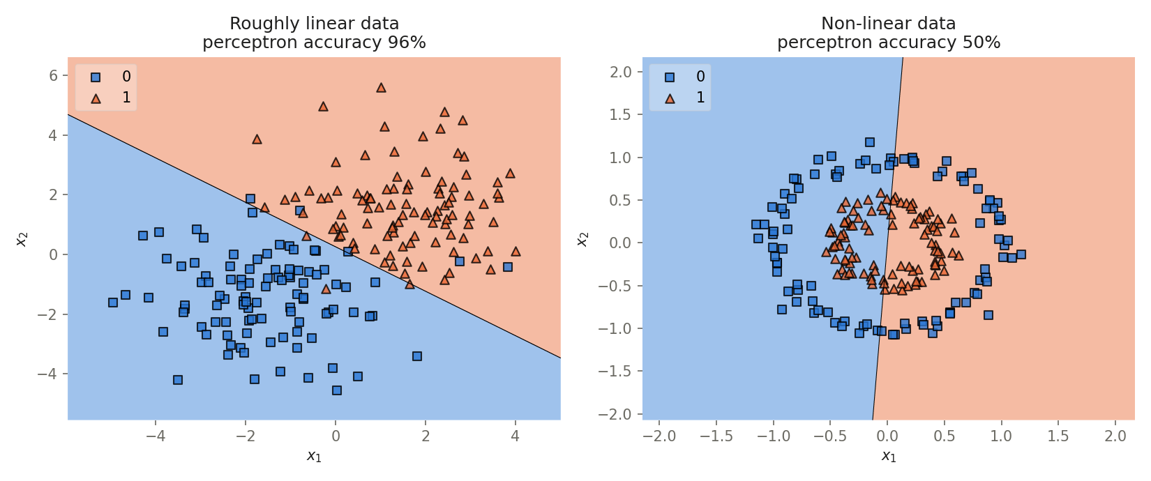

Left: two overlapping blob clusters split by a diagonal line, perceptron accuracy 96 percent. Right: one class forming a ring around the other, the perceptron's line cuts straight through both, accuracy 50 percent

On the roughly linear data the line gets 96% of points right; the few mistakes are points sitting inside the other cluster. On the ring data it does no better than a coin flip, at 50%: any straight line cuts through both classes. This holds in any number of dimensions: a plane or hyperplane is still flat. It's the main reason the perceptron on its own never became very powerful, and the problem multilayer perceptrons were built to solve.

6. A Perceptron in Code

Let's make all this concrete in code. The source notebook uses a small placement dataset: 100 students, each with a CGPA, a resume score (both roughly between 0 and 10) and whether they were placed. scikit-learn ships a Perceptron class, so there's nothing to write from scratch.

import numpy as np
import pandas as pd
import seaborn as sns
import matplotlib.pyplot as plt
 
df = pd.read_csv('placement.csv')
print(df.shape)
df.head()

(100, 3)
   cgpa  resume_score  placed
0  8.14          6.52       1
1  6.17          5.17       0
2  8.27          8.86       1
3  6.88          7.27       1
4  7.52          7.30       1

sns.scatterplot(x=df['cgpa'], y=df['resume_score'], hue=df['placed'])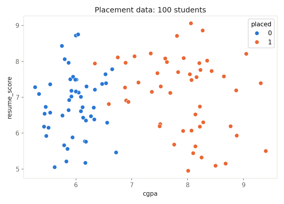

Scatter plot of resume score against CGPA for 100 students: unplaced students cluster at CGPA below about 6.7, placed students at higher CGPA, with resume scores spread across both groups

The data is roughly linearly separable, so a perceptron should be a reasonable fit. Look closely, though: almost all the separation is along CGPA. Unplaced students sit below a CGPA of about 6.7 and placed students mostly above it, while resume scores span the same range in both groups. Keep that in mind for the results below.

The perceptron will find a line through this plot, and in doing so it learns three numbers: $w_1$ for CGPA, $w_2$ for resume score, and $b$ .

X = df.iloc[:, 0:2]
y = df.iloc[:, -1]
 
from sklearn.linear_model import Perceptron
p = Perceptron()
p.fit(X, y)
 
p.coef_       # array([[ 40.26, -36.  ]])
p.intercept_  # array([-25.])

coef_ holds the weights and intercept_ holds the bias: $w_1 = 40.26$ , $w_2 = -36$ , $b = -25$ . To see the line, mlxtend can plot the two decision regions:

from mlxtend.plotting import plot_decision_regions
plot_decision_regions(X.values, y.values, clf=p, legend=2)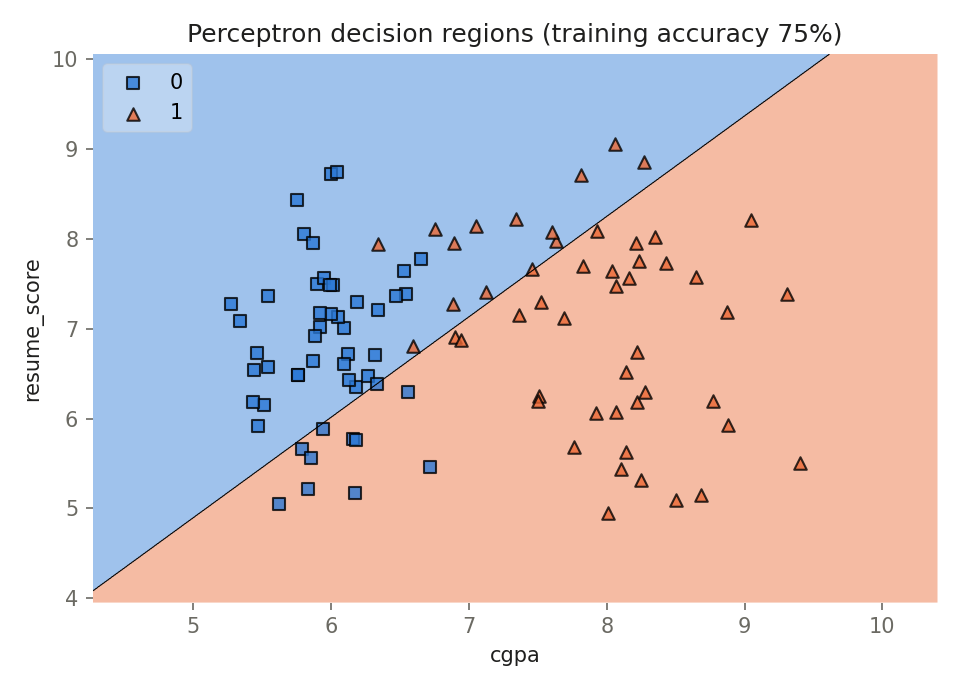

Perceptron decision regions on the placement data: a line rising from bottom left to top right, with the placed region below and right of it. Several unplaced students with low resume scores fall in the placed region and several placed students with high resume scores fall above the line

Reading the result

The numbers tell you everything about this line, so it's worth reading them before looking at the plot:

z = 40.26 \cdot \text{cgpa} - 36 \cdot \text{resume\_score} - 25

Which side is "placed"? Wherever $z \ge 0$ . A higher CGPA raises $z$ and a higher resume score lowers it, so the placed region is high CGPA and low resume score: below and to the right of the line. Setting $z = 0$ gives the line itself, $\text{resume\_score} \approx 1.12 \cdot \text{cgpa} - 0.69$ .
What the negative weight claims: that a better resume makes placement less likely. Nothing in the data supports that; resume score is barely related to placement here.
What it costs: the line gets only 75% of the training students right. Eleven unplaced students with low resume scores land on the "placed" side, and fourteen placed students with high resume scores land above the line.

So why did the perceptron settle on this line? Because a perceptron isn't looking for the best line. As you'll see in the next post, training simply nudges the line whenever it misclassifies a point, and stops once it decides it's no longer improving. Here, with default settings and unscaled features, scikit-learn stopped after just 7 passes over the data, and this is where the line happened to be. Nothing was tuned, and the dataset is tiny. The point of this example isn't the most accurate perceptron possible; it's seeing that fit really does produce a $w_1$ , a $w_2$ and a $b$ , and that those three numbers really are a line splitting the plane into two regions.

A good exercise: pick a dataset with more than two input columns, apply a perceptron to it, and check its accuracy.

Wrapping Up

A perceptron is a supervised learning algorithm and the building block of neural networks. It computes a weighted sum $z = w_1 x_1 + w_2 x_2 + \dots + b$ and passes it through an activation function; here, the step function, which outputs 1 if $z \ge 0$ and 0 otherwise.
Training finds the weights and bias; prediction just plugs a new example into the weighted sum and applies the threshold. More input columns means more inputs and weights, nothing else.
A perceptron is weakly inspired by a biological neuron (dendrites, nucleus, axon map roughly to inputs, processing, output) but is far simpler, has a fully known internal computation, and has no neuroplasticity.
Weights can be read as feature importance, but only once the features are on the same scale.
Geometrically, a perceptron is a line in 2D, a plane in 3D and a hyperplane beyond that, splitting space into two regions: a binary classifier. The weights set the boundary's tilt and the bias shifts it.
Its big limitation: it can only handle linear or roughly linear data. On non-linear data like concentric rings, accuracy falls to chance.
In scikit-learn, Perceptron().fit gives you coef_ (weights) and intercept_ (bias). Read their signs to see which side is which class, and don't assume the line is the best possible one.

Next up: how a perceptron is actually trained.

View all chapters in Deep Learning →